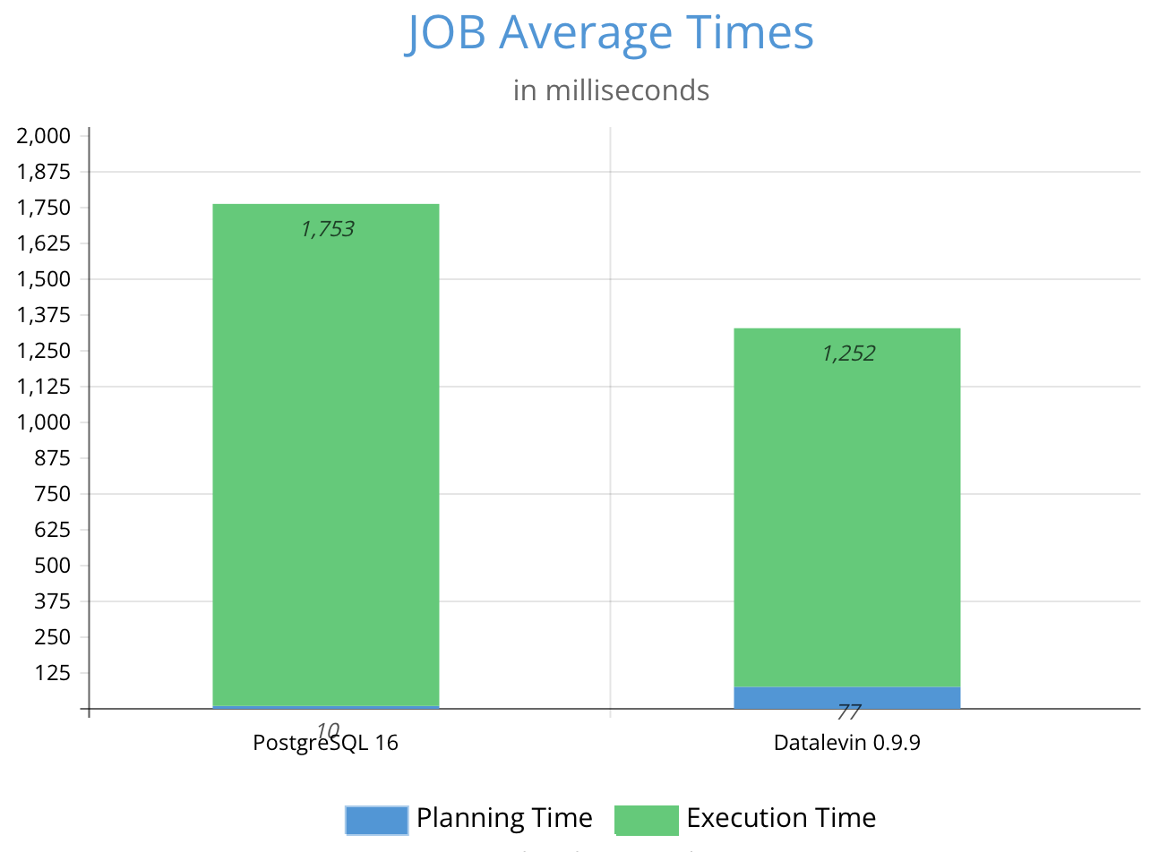
This is a post about Datalevin, an open-source database system that I have been building since 2020. Although JOB here is really an acronym for Join Order Benchmark, a benchmark for complex database queries, I intend to build up Datalevin to compete for the same kind of jobs usually held by a RDBMS. I hope this title is received well and not seen as just a pun :-). This post describes my journey in making Datalevin competitive in the JOB benchmark, where it outperformed PostgreSQL by a small margin.
Datalevin is a triplestore, which
means it stores data in units of three elements known as triples. Specifically,
the three elements are entity (E), attribute (A) and value (V). For
example, to store a piece of information: a person is named "John Smith", E
would be the entity id number of this person, A would be an attribute named
:person/name , and V would be "John Smith", the attribute value of
the entity.
Unlike what the Wikipedia page of triplestore seems to suggest, a triplestore is not necessarily about Semantic Web use cases. Datalevin is a general purpose database system that follows an approach pioneered by Datomic, and uses its flavor of Datalog as the query language.
Why Datalog?
The flavor of Datalog used in Datalevin can be considered a modern alternative to SQL.
There have been many articles discussing the limitations of SQL as a database query language, such as Against SQL and We can do better than SQL, and I am sympathetic towards those views and recommend readers to look into them.
One point I would like to add, from a point of view of human computer interaction, is related to the historical context of SQL [1]. As one of those ALL CAP languages (e.g. COBOL), SQL was from an era when enthusiastic computer scientists believed that structured English could be a good human interface to computers. The rationale was that business people could be taught to use such languages to communicate with computers. We all know how that turned out: business people are allergic to any kind of formal languages, i.e. code, so these languages still end up as tools for programmers only. However, structured English makes for poor programming languages, because it is difficult to parse, compose or extend. SQL is the most stubborn left-over from those ill-considered experiments, perhaps due to the fact that data often last longer than programs.
Datalog used in Datalevin does not have such historical baggage. Let us look at an example:
;; query about persons who are adult males, whose name ends with Smith

[:find ?name
 :where
 [?person :person/age ?age]
 [?person :person/name ?name]
 [(like ?name "%Smith")]
 [(<= 18 ?age)]]
Similar to SQL's SELECT and WHERE, this flavor of Datalog has explicit
:find and :where sections, so it is easier to grok than the original Datalog
syntax from Prolog, which read like math expressions. Unlike SQL though, this
query language is represented as a data structure in
EDN format, which is amicable to
programmatic manipulation, just like JSON.
Each where clause is delimited by a pair of [ ]. All the where clauses are
AND'ed together, i.e. they all must evaluate to be true for the query to return
non-empty results. There are two types of where clauses in this query: triple
patterns and predicates.
Just like a triple, a triple pattern consists of Entity (E), Attribute (A) and
Value (V), in that order. Any of the three elements could be a variable, which
is a user defined symbol starting with a ?. For example, triple pattern
[?person :person/age 18] says that there are entities that we name with a
variable ?person, and they have an attribute :person/age with the value
18. Triple patterns must match with the data, so that variables can be bound
with values from the database. For this pattern, ?person would be bound with
entity IDs of all persons aged 18 in the database.
Predicates are boolean functions, and they are enclosed in a pair of ( ).
The first element inside the parentheses is the function name, e.g. like,
<=, and so on, and the rest are the function arguments. All the predicates must
evaluate to be true for the query to return non-empty results.
That's it, the syntax of Datalevin's Datalog. There are neither complex syntactic rules, nor hundreds of reserved words.
More importantly, Datalog is very high level and truly declarative. It does not expose low level technical details of database operations to the users, nor requires the users to speak database jargons or be a relational algebra expert to use the language well. For example, the user is not required to understand the concept of joins, let alone the many different types of joins: inner, left, right, full, self joins, etc.
Joins are implicit in Datalog and are completely oblivious for the users. All users need to focus on are the logic relationships in their data, the rest is left for the database system to figure out. Datalog greatly simplifies the writing of complex queries. This is perhaps the main strength of this query language. My experience in onboarding new users has been that it normally took people less than half an hour to become a competent Datalog query writer.
Regardless the language level differences, Datalog in Datalevin is still backed up by a computational substrate based on relational algebra. It just treats relational algebra as underlying implementation details that users should not be concerned with.
Why a triple store?
When people talk about relational databases, they often assume it's a row store or a column store, as if relational algebra has something to do with how a table is stored. But, it doesn't. As a mathematical theory, relational algebra does not specify how a relation should be stored in computers. Therefore, in addition to storing a relation as rows or columns, storing it as triples are equally sound, if not better.

For example, for the data set above, a row store would store them as two tables.
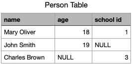
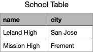
Storing a table as triples means storing the table as a list of table cells, i.e. as a list of the smallest identifiable units of the table.
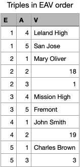
Storing table cells as rows or columns are just two concrete ways of bundling the table cells together for efficiency purpose, so that column identifiers or row identifier would not need to be repeated. That is to say, they are optimizations. So, the question is, are these "premature optimizations"?
I argue that they are. One problem with fixating the storage to either a row or a column format, is that it impedes querying the data later on. Specifically, it makes the work of query optimizer unnecessarily hard.
Essentially, both row and column storage are place oriented: table cells are
identified by positions, rather than by explicit identifiers. One consequence is
that missing data cells still have to be represented positionally, i.e. they
need to take up places. RDBMS normally store these as special null values.
This is what complicates the collection of statistics of table cells, which a
query optimizer demands: it needs to know how many non-null data points it is
dealing with under all kinds of conditions. The place based storage does not
have a cheap way of providing this information, because any position could hold
a null value, or not.
To work around this problem, RDBMS resorts to expensive and complicated processes to collect various approximations of exact data counts, e.g. histograms. Still, the lack of direct information often forces the optimizer to make unrealistically simplistic statistical assumptions about data distribution, e.g. independence, uniformity, and so on. This so called "cardinality estimation" problem is such a notoriously hard topic in database research that it is sometimes called "Achilles Heel" of database query processing [2].
In a triplestore, each table cell is identified explicitly by both row and
column, e.g. E is the row, A is the column, and V is the value. A triple
alone has complete information about a piece of data. Hence, a triple is called
a datom (data atom) in this flavor of Datalog. Some simplifications
naturally arise in such a triplestore.
In a triplestore, a missing table cell is simply missing from the storage:
null is not stored, and absence means null. To remove a piece of data, one
actually removes it from the storage, instead of setting some values to
null. This is a critical simplification that enables easy and accurate counting
of non-null data in the database.
Another simplification is that the entire database is essentially just one big
table. E and A are all globally scoped. In Datalevin, E is represented as
a 64 bit integer, and A a 32 bit integer. Database schema specifies only
information about each attribute, e.g. its id, data type, uniqueness, and so on.
;; Datalevin schema for the example data above

{:person/name   {:db/aid 1 :db/valueType :db.type/string}
 :person/age    {:db/aid 2 :db/valueType :db.type/long}
 :person/school {:db/aid 3 :db/valueType :db.type/ref}
 :school/name   {:db/aid 4 :db/valueType :db.type/string}
 :school/city   {:db/aid 5 :db/valueType :db.type/string}}
Information about individual tables are no longer necessary. Name
spaced attribute names still allow grouping of attributes, e.g. :person/name,
person/age are attributes of person entity, but this is just a convention,
not a physically separated table. Tables dedicated to joins also disappear, as
they are simply handled by attributes with entity id as values (i.e. of
reference data type: :db.type/ref).
The atomic nature of a datom allows maximum flexibility, as these datoms can be
arranged in ways that facilitate querying them. For example, if datoms are
ordered by E first, then A, then V, one essentially gets a row major
storage that has the similar properties of a row store. If datoms are ordered by
A first, one gets a column major storage that has the same advantage of a
column store. Tripestores often store data in both orderings, so that
essentially all data are indexed by default. Not having to manage indices can
save some headache.
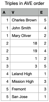
Obviously, the storage of triplestores is redundant, as row identifiers and column identifiers are repeated. If storing both row major and column major data ordering, even more storage spaces are taken. More data means higher I/O demand, and slower querying may be resulted. This is perhaps the main challenge that has prevented the widespread use of triplestores.
I argue that this data storage redundancy problem is easier to mitigate than the
hard problem of cardinality estimation resulted from bundling table cells as
rows or columns. For example, prefix compression could be used to minimize the
repetition. Datalevin utilizes this strategy by storing data in a two level
nesting schema: AV is nested underneath E in EAV ordering, and E
underneath AV in AVE ordering. Obviously, three level nesting can further
reduce data redundancy.
Critically, with unbundled table cells in triplestores, the problem of cardinalty estimation can be solved with straightforward counting or sampling. I argue that this advantage is perhaps a good reason to use a triplestore. As a demonstration, Datalevin employed this simple strategy of counting and sampling to achieve better performance than PostgreSQL in JOB benchmark.
Join Order Benchmark (JOB)
This benchmark aims to test a database query optimizer's capacity to handle complex queries that involve many joins [3]. Based on Internet Movie Database, 113 analytical SQL queries were developed to have between 3 and 16 joins, with an average of 8 joins per query. These SQL queries were translated into the equivalent Datalevin queries, which were verified to produce exactly the same results as corresponding SQL ones.
The tests were conducted on a MacBook Pro Nov 2023, Apple M3 Pro chip, 6 performance cores and 6 efficiency cores, 36GB memory, and 1TB SSD disk.
On average, Datalevin is about 1.3 times faster than PostgreSQL 16 in this benchmark. More details can be found here.
Analysis
Given that Datalevin is written in Clojure — a functional programming language on JVM, not widely known for speed, and PostgreSQL is written in highly optimized C code, it's clear that the query optimizer of Datalevin generates better execution plans than that of PostgreSQL on average.
As I will show with an example, Datalevin's better plan is mainly achieved by having more accurate estimate of result sizes at each execution step, corroborating with the point argued above regarding the superiority of triplestores.
Query 20a of JOB is what PostgreSQL did the worst compared with Datalevin. It took PostgreSQL over a minute to execute its plan whereas Datalevin took about a second. Let us look at the SQL query first.
-- query 20a

SELECT MIN(t.title) AS complete_downey_ironman_movie
FROM complete_cast AS cc,
     comp_cast_type AS cct1,
     comp_cast_type AS cct2,
     char_name AS chn,
     cast_info AS ci,
     keyword AS k,
     kind_type AS kt,
     movie_keyword AS mk,
     name AS n,
     title AS t
WHERE cct1.kind = 'cast'
  AND cct2.kind LIKE '%complete%'
  AND chn.name NOT LIKE '%Sherlock%'
  AND (chn.name LIKE '%Tony%Stark%'
       OR chn.name LIKE '%Iron%Man%')
  AND k.keyword IN ('superhero',
                    'sequel',
                    'second-part',
                    'marvel-comics',
                    'based-on-comic',
                    'tv-special',
                    'fight',
                    'violence')
  AND kt.kind = 'movie'
  AND t.production_year > 1950
  AND kt.id = t.kind_id
  AND t.id = mk.movie_id
  AND t.id = ci.movie_id
  AND t.id = cc.movie_id
  AND mk.movie_id = ci.movie_id
  AND mk.movie_id = cc.movie_id
  AND ci.movie_id = cc.movie_id
  AND chn.id = ci.person_role_id
  AND n.id = ci.person_id
  AND k.id = mk.keyword_id
  AND cct1.id = cc.subject_id
  AND cct2.id = cc.status_id;
The PostgreSQL EXPLAIN ANALYZE output for this query:
                                                                                          QUERY PLAN
-----------------------------------------------------------------------------------------------------------------------------------------------------------------------------------------------
 Nested Loop  (cost=21.78..2474.54 rows=1 width=17) (actual time=17052.871..72628.822 rows=33 loops=1)
   ->  Nested Loop  (cost=21.35..2474.09 rows=1 width=21) (actual time=17052.352..72626.880 rows=33 loops=1)
         ->  Nested Loop  (cost=20.93..2473.63 rows=1 width=25) (actual time=17042.110..72584.290 rows=1314 loops=1)
               ->  Nested Loop  (cost=20.50..2473.17 rows=1 width=29) (actual time=1.352..35903.879 rows=87986607 loops=1)
                     Join Filter: (ci.movie_id = t.id)
                     ->  Nested Loop  (cost=20.06..2471.42 rows=1 width=33) (actual time=1.124..3346.138 rows=978322 loops=1)
                           ->  Nested Loop  (cost=19.63..2469.68 rows=1 width=25) (actual time=0.703..2394.487 rows=28583 loops=1)
                                 ->  Nested Loop  (cost=19.48..2469.50 rows=1 width=29) (actual time=0.688..2362.288 rows=73560 loops=1)
                                       ->  Nested Loop  (cost=19.05..2467.72 rows=1 width=4) (actual time=0.444..41.257 rows=85941 loops=1)
                                             ->  Hash Join  (cost=18.89..2462.46 rows=190 width=8) (actual time=0.416..22.960 rows=135086 loops=1)
                                                   Hash Cond: (cc.status_id = cct2.id)
                                                   ->  Seq Scan on complete_cast cc  (cost=0.00..2086.86 rows=135086 width=12) (actual time=0.365..6.616 rows=135086 loops=1)
                                                   ->  Hash  (cost=18.88..18.88 rows=1 width=4) (actual time=0.035..0.035 rows=2 loops=1)
                                                         Buckets: 1024  Batches: 1  Memory Usage: 9kB
                                                         ->  Seq Scan on comp_cast_type cct2  (cost=0.00..18.88 rows=1 width=4) (actual time=0.027..0.028 rows=2 loops=1)
                                                               Filter: ((kind)::text ~~ '%complete%'::text)
                                                               Rows Removed by Filter: 2
                                             ->  Memoize  (cost=0.16..0.18 rows=1 width=4) (actual time=0.000..0.000 rows=1 loops=135086)
                                                   Cache Key: cc.subject_id
                                                   Cache Mode: logical
                                                   Hits: 135084  Misses: 2  Evictions: 0  Overflows: 0  Memory Usage: 1kB
                                                   ->  Index Scan using comp_cast_type_pkey on comp_cast_type cct1  (cost=0.15..0.17 rows=1 width=4) (actual time=0.119..0.119 rows=0 loops=2)
                                                         Index Cond: (id = cc.subject_id)
                                                         Filter: ((kind)::text = 'cast'::text)
                                                         Rows Removed by Filter: 0
                                       ->  Index Scan using title_pkey on title t  (cost=0.43..1.78 rows=1 width=25) (actual time=0.027..0.027 rows=1 loops=85941)
                                             Index Cond: (id = cc.movie_id)
                                             Filter: (production_year > 1950)
                                             Rows Removed by Filter: 0
                                 ->  Index Scan using kind_type_pkey on kind_type kt  (cost=0.15..0.17 rows=1 width=4) (actual time=0.000..0.000 rows=0 loops=73560)
                                       Index Cond: (id = t.kind_id)
                                       Filter: ((kind)::text = 'movie'::text)
                                       Rows Removed by Filter: 1
                           ->  Index Scan using movie_id_movie_keyword on movie_keyword mk  (cost=0.43..1.29 rows=46 width=8) (actual time=0.024..0.031 rows=34 loops=28583)
                                 Index Cond: (movie_id = t.id)
                     ->  Index Scan using movie_id_cast_info on cast_info ci  (cost=0.44..1.31 rows=35 width=12) (actual time=0.001..0.028 rows=90 loops=978322)
                           Index Cond: (movie_id = mk.movie_id)
               ->  Index Scan using char_name_pkey on char_name chn  (cost=0.43..0.46 rows=1 width=4) (actual time=0.000..0.000 rows=0 loops=87986607)
                     Index Cond: (id = ci.person_role_id)
                     Filter: ((name !~~ '%Sherlock%'::text) AND ((name ~~ '%Tony%Stark%'::text) OR (name ~~ '%Iron%Man%'::text)))
                     Rows Removed by Filter: 0
         ->  Index Scan using keyword_pkey on keyword k  (cost=0.42..0.45 rows=1 width=4) (actual time=0.032..0.032 rows=0 loops=1314)
               Index Cond: (id = mk.keyword_id)
               Filter: (keyword = ANY ('{superhero,sequel,second-part,marvel-comics,based-on-comic,tv-special,fight,violence}'::text[]))
               Rows Removed by Filter: 1
   ->  Index Only Scan using name_pkey on name n  (cost=0.43..0.45 rows=1 width=4) (actual time=0.059..0.059 rows=1 loops=33)
         Index Cond: (id = ci.person_id)
         Heap Fetches: 0
 Planning Time: 28.727 ms
 Execution Time: 72629.051 ms
(50 rows)
As can be seen, the catastrophic running time is mainly due to vastly
underestimated result join sizes, leading to sub-optimal join order. For
instance, the planner estimated that the hash join of complete_cast and
comp_cast_type would produce 190 rows but actually got 135086 rows. Similar
under-estimation is persisted and its effect accumulated, eventually reaching a
staggering 1 vs. 87986607 discrepancy with actual result size.
These underestimations are due to the strong statistical assumptions its estimator makes: value uniformity and column independence. However, the actual value distribution is highly skewed and the columns are highly correlated with one another, as it is often the case in real world datasets. I would like to point out that this problem is not unique to PostgreSQL, but in fact common in all row based RDBMS [3]. These strong assumptions are necessary because more direct information is not available in row stores.
Datalevin does not rely on such strong statistical assumptions to estimate join result size. Instead, it simply counts or samples to obtain the base selectivity ratios. Then, for each pair of base relations, it actually executes the joins using the samples, and thus obtains the pair-wise join selectivity ratios. These ratios are simply used in estimation of join sizes in later joins. The only assumption it makes is that the selectivity ratios of pair-wise joins are similar to those of later joins. If the samples are representative, this assumption would not be too off base.
For query 20a, the corresponding Datalog query is the following:
;; query 20a

 [:find (min ?t.title)
  :where
  [?cct1 :comp-cast-type/kind "cast"]
  [?cct2 :comp-cast-type/kind ?cct2.kind]
  [(like ?cct2.kind "%complete%")]
  [?chn :char-name/name ?chn.name]
  [(not-like ?chn.name "%Sherlock%")]
  [(or (like ?chn.name "%Tony%Stark%") (like ?chn.name "%Iron%Man%"))]
  [?k :keyword/keyword ?k.keyword]
  [(in ?k.keyword ["superhero", "sequel", "second-part",
                  "marvel-comics", "based-on-comic",
                  "tv-special", "fight", "violence"])]
  [?kt :kind-type/kind "movie"]
  [?t :title/production-year ?t.production-year]
  [(< 1950 ?t.production-year)]
  [?t :title/kind ?kt]
  [?mk :movie-keyword/movie ?t]
  [?ci :cast-info/movie ?t]
  [?cc :complete-cast/movie ?t]
  [?ci :cast-info/person-role ?chn]
  [?ci :cast-info/person ?n]
  [?mk :movie-keyword/keyword ?k]
  [?cc :complete-cast/subject ?cct1]
  [?cc :complete-cast/status ?cct2]
  [?t :title/title ?t.title]]
The :plan portion of the explain output is the following:
  [[{:steps       ["Initialize [?k ?k.keyword] by range [[[:closed \"based-on-comic\"] [:closed \"based-on-comic\"]] [[:closed \"fight\"] [:closed \"fight\"]] [[:closed \"marvel-comics\"] [:closed \"marvel-comics\"]] [[:closed \"second-part\"] [:closed \"second-part\"]] [[:closed \"sequel\"] [:closed \"sequel\"]] [[:closed \"superhero\"] [:closed \"superhero\"]] [[:closed \"tv-special\"] [:closed \"tv-special\"]] [[:closed \"violence\"] [:closed \"violence\"]]] on :keyword/keyword."],
     :cost        17,
     :size        8,
     :actual-size 8}
    {:steps       ["Merge ?mk by reverse reference of :movie-keyword/keyword."
                   "Merge [?t] by scanning [:movie-keyword/movie]."],
     :cost        41,
     :size        35549,
     :actual-size 35548}
    {:steps       ["Merge ?cc by equal values of :complete-cast/movie."
                   "Merge [?cct2 ?cct1] by scanning [:complete-cast/status :complete-cast/subject]."],
     :cost        147569,
     :size        11909,
     :actual-size 12810}
    {:steps       ["Merge ?ci by equal values of :cast-info/movie."
                   "Merge [?chn ?n] by scanning [:cast-info/person-role :cast-info/person]."],
     :cost        196991,
     :size        472311,
     :actual-size 476091}
    {:steps       ["Merge [?chn.name] by scanning [:char-name/name]."],
     :cost        2180697,
     :size        472,
     :actual-size 33}
    {:steps       ["Merge [?t.title ?kt ?t.production-year] by scanning [:title/title :title/kind :title/production-year]."],
     :cost        2184661,
     :size        472,
     :actual-size 33}
    {:steps       ["Filter by predicates on [:comp-cast-type/kind]."],
     :cost        2186643,
     :size        472,
     :actual-size 33}
    {:steps       ["Filter by predicates on [:kind-type/kind]."],
     :cost        2188625,
     :size        472,
     :actual-size 33}
    {:steps       ["Merge [?cct2.kind] by scanning [:comp-cast-type/kind]."],
     :cost        2190607,
     :size        472,
     :actual-size 33}]]
As can be seen, the estimated join sizes are close to the actual sizes. Particularly for the initial steps, the estimations are almost exact. For data sizes that smaller than a user configured threshold, actual counting of the data is performed, while sampling was performed for larger data sizes. Both are performed under query specific conditions.
Compared with the tree shape of the PostgreSQL's plan, the plan in Datalevin is linear, because we only consider left-deep join tree. We join one base relation at a time in order to take advantage of the accurate counting and sampling of base relations.
Counting and sampling under query conditions are straightforward in Datalevin,
thanks to the nested triple storage. Applicable value predicates are translated
into range queries in AVE ordering of triples. When both A and V are known,
obtaining the count is a constant time operation. When V is a range, the count
is just the sum of the counts in range; The only missing information is the total
count of A, which is easily maintained during transaction.
More details of the Datalevin query planner and execution engine can be found here.
Summary
With Datalevin, I have demonstrated that a triplestore has some unique advantages compared with row or column based databases. It helps with solving the difficult problem of cardinality estimation, while its shortcomings can be easily mitigated by nested storage of triples. Paired with a Datalog query language, it makes a promising choice as a modern alternative to SQL RDBMS, as it is much more ergonomic.
References
[1] Chamberlin, D. and Boyce, R.. "SEQUEL: A Structured English Query Language", Proc. ACM SIGFIDET Workshop on Data Description Access and Control. 1974.
[2] Leis, V., et al. "Cardinality Estimation Done Right: Index-Based Join Sampling." Cidr. 2017.
[3] Leis, V., et al. "How good are query optimizers, really?." VLDB Endowment. 2015.
 yyhh.org
Comments
comments powered by Disqus